Python量化因子测算与绘图超详细流程代码

量化因子的测算通常都是模拟交易，计算各种指标，其中：

• 测算需要用到的第三方库：numpy，pandas，talib
• 绘图需要用到的第三方库：matplotlib，seaborn

其他库随策略的需要额外添加

因子测算框架

这里博主分享自己测算时常使用的流程，希望与大家共同进步！

测算时从因子到收益的整个流程如下：策略（因子组合） -> 买卖信号 -> 买点与卖点 -> 收益

因此我们在测算时，针对每一个个股：

1. 预处理股票数据

首先这里是常用的一个工具导入，包括测算用的库与绘图用的库（含图片中文显示空白解决方案）

# 测算用

import numpy as np

import pandas as pd

from copy import deepcopy

from tqdm import tqdm

from datetime import datetime

import talib

# 绘图用

import matplotlib as mpl

import matplotlib.pyplot as plt

import seaborn as sns

%matplotlib inline

# 绘图现实中文

sns.set()

plt.rcParams["figure.figsize"] = (20,10)

plt.rcParams['font.sans-serif'] = ['Arial Unicode MS']  # 当前字体支持中文

plt.rcParams['axes.unicode_minus'] = False  # 解决保存图像是负号'-'显示为方块的问题

# 其他

import warnings

warnings.filterwarnings("ignore")

然后是循环读取股票的代码：

import os

def readfile(path, limit=None):

    files = os.listdir(path)

    file_list = []

    for file in files:  # 遍历文件夹

        if not os.path.isdir(file):

            file_list.append(path + '/' + file)

    if limit:

        return file_list[:limit]

    return file_list

stock_dict = {}

for _file in tqdm(readfile("../data/stock_data")):

    if not _file.endswith(".pkl"):

        continue

    # TODO 这里可以添加筛选，是否需要将当前的股票添加到测算的股票池中

    file_df = pd.read_pickle(_file)

    file_df.set_index(["日期"], inplace=True)

    file_df.index.name = ""

    file_df.index = pd.to_datetime(file_df.index)

    file_df.rename(columns={'开盘':'open',"收盘":"close","最高":"high","最低":"low","成交量":"volume"},inplace=True)

    stock_code = _file.split("/")[-1].replace(".pkl", '')

    # TODO 这里可以添加日期，用来截取一部分数据

    stock_dict[stock_code] = file_df

上面一部分是处理股票数据，处理后的数据都会保存在 stock_dict 这个变量中，键是股票的代码，值是股票数据

2. 指标测算

测算指标时，我们以一只股票为例：

for _index,_stock_df in tqdm(stock_dict.items()):

    measure_df = deepcopy(_stock_df)

代码中的：

• 这里的measure_df即要测算的dataframe数据
• 使用deepcopy是防止测算的过程影响到原始数据

然后我们就可以循环这一个股票的每一行（代表每一天），测算的交易规则如下：

• 买入规则：买入信号发出&当前没有持仓，则买入
• 卖出规则：卖出信号发出&当前有持仓，则卖出

# 开始测算

trade_record_list = []

this_trade:dict = None

for _mea_i, _mea_series in measure_df.iterrows(): # 循环每一天

    if 发出买入信号:

        if this_trade is None:  # 当前没有持仓，则买入

            this_trade = {

                "buy_date": _mea_i,

                "close_record": [_mea_series['close']],

            }

    elif 发出卖出信号:

        if this_trade is not None:  # 要执行卖出

            this_trade['sell_date'] = _mea_i

            this_trade['close_record'].append(_mea_series['close'])

            trade_record_list.append(this_trade)

            this_trade = None

    else:

        if this_trade is not None:  # 当前有持仓

            this_trade['close_record'].append(_mea_series['close'])

上述代码中，我们将每一个完整的交易（买->持有->卖），都保存在了trade_record_list变量中，每一个完整的交易都会记录：

{

    'buy_date': Timestamp('2015-08-31 00:00:00'), # 买入时间

    'close_record': [41.1,42.0,40.15,40.65,36.6,32.97], # 收盘价的记录

    'sell_date': Timestamp('2015-10-12 00:00:00')} # 卖出时间

    # TODO 也可以添加自定义记录的指标

}

3. 测算结果整理

直接使用 pd.DataFrame(trade_record_list)，就可以看到总的交易结果：

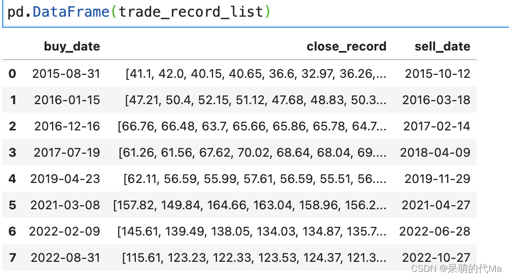
整理的过程也相对简单且独立，就是循环这个交易，然后计算想要的指标，比如单次交易的年化收益可以使用：

trade_record_df = pd.DataFrame(trade_record_list)

for _,_trade_series in trade_record_df.iterrows():

    trade_record_df.loc[_i,'年化收益率'] = (_trade_series['close_record'][-1] - _trade_series['close_record'][0])/_trade_series['close_record'][0]/(_trade_series['sell_date'] - _trade_series['buy_date']).days * 365 # 年化收益

    # TODO 这里根据自己想要的结果添加更多的测算指标

4. 结果绘图

绘图的代码通常比较固定，比如胜率图：

# 清理绘图缓存

plt.cla()

plt.clf()

# 开始绘图

plt.figure(figsize=(10, 14), dpi=100)

# 使用seaborn绘制胜率图

fig = sns.heatmap(pd.DataFrame(total_measure_record).T.round(2), annot=True, cmap="RdBu_r",center=0.5)

plt.title("胜率图")

scatter_fig = fig.get_figure()

# 保存到本地

scatter_fig.savefig("胜率图")

scatter_fig.show() # 最后显示