数据集利用的是CPSC2020数据集。
训练数据包括从心律失常患者收集的10个单导联心电图记录,每个记录持续约24小时。

下载完成后的TrainingSet数据集包括两个文件夹,分别是data和ref。data和ref文件夹内分别有10个mat文件。
采样率为 400。
数据集链接如下:http://2020.icbeb.org/CSPC2020
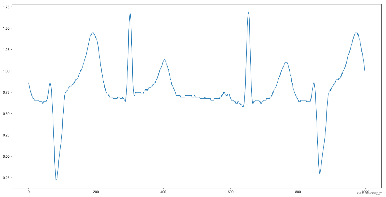
查看一下前1000个心电图数据:
datafile = 'E:/Wendy/Desktop/TrainingSet/data/A04.mat'# 采样率400

data = scio.loadmat(datafile)

#rint(data) # dict


sig = data['ecg']# (x,1)

#print(sig)

sig = np.reshape(sig,(-1)) # (x,)转换为一维向量

print(sig)

sigPlot = sig[1:5*200]# # 获取前1000个信号

fig = plt.figure(figsize=(20, 10),dpi=400)

plt.plot(sigPlot)

plt.show()
运行结果:
将标签数据转化为一维向量
datafile = 'E:/Wendy/Desktop/TrainingSet/ref/R04.mat'# 采样率400

data = scio.loadmat(datafile)

#print(data)

label = data['ref'][0][0]

S_ref = label[0];

S_ref = np.reshape(S_ref,(-1)) # 转换为一维向量

V_ref = label[1];

V_ref = np.reshape(V_ref,(-1)) # 转换为一维向量
数据分割为5s一个片段
思路:房早室早心拍和前后两个心拍均有关系,按照平均心率72计算,平均每个心拍的时间为60/72,因此5个心拍的时间为60/725=4.1667 4.1667s不好计算,故选择5s 5 ( 秒 ) s a m p r = 5 ∗ 400 = 2000 个 s a m p l e 5(秒)sampr = 5*400=2000个sample5(秒)sampr=5∗400=2000个sample
定义标签:0:其他;1:V_ref; 2:S_ref;
a = len(sig)

Fs = 400 # 采样率为400

segLen = 5*Fs # 2000

num = int(a/segLen)

print(num)
运行结果:
17650
其中Fs为采样率,segLen为片段长度,num为片段数量。
接下来需要整合数据和标签:
all_data=[]

all_label = [];

i=1

while i<num+1:

    all_data.append(np.array(sig[(i-1)*segLen:i*segLen]))

    # 标签

    if set(S_ref) & set(range((i-1)*segLen,i*segLen)):

        all_label.append(2)

    elif set(V_ref) & set(range((i-1)*segLen,i*segLen)):

        all_label.append(1)

    else:

        all_label.append(0)

    i=i+1

type(all_data)# list类型

type(all_label)# list类型

print((np.array(all_data)).shape) # 17650为数据长度,2000为数据个数

print((np.array(all_label)).shape)

#print(all_data)
运行结果:
(17650, 2000)
(17650,)
17650为数据长度,2000为数据个数。
将数据保存为字典类型:
import pickle

res = {'data':all_data, 'label':all_label} # 字典类型dict

with open('./cpsc2020.pkl', 'wb') as fout: # #将结果保存为cpsc2020.pkl

    pickle.dump(res, fout)
将数据归一化并进行标签编码,划分训练集和测试集,训练集为90%,测试集为10%,打乱数据并将其扩展为二维:
import numpy as np

import pandas as pd

import scipy.io

from matplotlib import pyplot as plt

import pickle

from sklearn.model_selection import train_test_split

from collections import Counter

from tqdm import tqdm


def read_data_physionet():

    """

    only N V, S

    """

    # read pkl

    with open('./cpsc2020.pkl', 'rb') as fin:

        res = pickle.load(fin) # 加载数据集

    ## 数据归一化

    all_data = res['data']

    for i in range(len(all_data)):

        tmp_data = all_data[i]

        tmp_std = np.std(tmp_data) # 获取数据标准差

        tmp_mean = np.mean(tmp_data) # 获取数据均值

        if(tmp_std==0):   # i=1239-1271均为0

            tmp_std = 1

        all_data[i] = (tmp_data - tmp_mean) / tmp_std  # 归一化

    all_data = []

    ## 标签编码

    all_label = []

    for i in range(len(res['label'])):

        if res['label'][i] == 1:

            all_label.append(1)

            all_data.append(res['data'][i])

        elif res['label'][i] == 2:

            all_label.append(2)

            all_data.append(res['data'][i])

        else:

            all_label.append(0)

            all_data.append(res['data'][i])

    all_label = np.array(all_label)

    all_data = np.array(all_data)


    # 划分训练集和测试集,训练集90%,测试集10%

    X_train, X_test, Y_train, Y_test = train_test_split(all_data, all_label, test_size=0.1, random_state=15)


    print('训练集和测试集中 其他类别(0);室早(1);房早(2)的数量: ')

    print(Counter(Y_train), Counter(Y_test))


    # 打乱训练集

    shuffle_pid = np.random.permutation(Y_train.shape[0])

    X_train = X_train[shuffle_pid]

    Y_train = Y_train[shuffle_pid]


    # 扩展为二维(x,1)

    X_train = np.expand_dims(X_train, 1)

    X_test = np.expand_dims(X_test, 1)


    return X_train, X_test, Y_train, Y_test

X_train, X_test, Y_train, Y_test = read_data_physionet()
运行结果:
训练集和测试集中 其他类别(0);室早(1);房早(2)的数量:
Counter({1: 8741, 0: 4605, 2: 2539}) Counter({1: 1012, 0: 478, 2: 275})
自行构建数据集:
# 构建数据结构 MyDataset

# 单条数据信号的形状为:1*2000

import numpy as np

from collections import Counter

from tqdm import tqdm

from matplotlib import pyplot as plt

from sklearn.metrics import classification_report


import torch

import torch.nn as nn

import torch.optim as optim

import torch.nn.functional as F

from torch.utils.data import Dataset, DataLoader


class MyDataset(Dataset):

    def __init__(self, data, label):

        self.data = data

        self.label = label

    #把numpy转换为Tensor

    def __getitem__(self, index):

        return (torch.tensor(self.data[index], dtype=torch.float), torch.tensor(self.label[index], dtype=torch.long))


    def __len__(self):

        return len(self.data)
搭建CNN网络结构:
# 搭建神经网络

class CNN(nn.Module):

    def __init__(self):

        super(CNN, self).__init__()

        self.conv1 = nn.Sequential(         # input shape (1, 1, 2000)

            nn.Conv1d(

                in_channels=1,

                out_channels=16,

                kernel_size=5,

                stride=1,

                padding=2,

            ),                              # output shape (16, 1, 2000)

            nn.Dropout(0.2),

            nn.ReLU(),

            nn.MaxPool1d(kernel_size=5),    # choose max value in 1x5 area, output shape (16, 1, 400)2000/5

        )

        self.conv2 = nn.Sequential(         # input shape (16, 1, 400)

            nn.Conv1d(16, 32, 5, 1, 2),     # output shape (32, 1, 400)

            nn.Dropout(0.2),

            nn.ReLU(),

            nn.MaxPool1d(kernel_size=5),    # output shape (32, 1, 400/5=80)

        )

        self.out = nn.Linear(32 *  80, 3)   # fully connected layer, output 3 classes


    def forward(self, x):

        x = self.conv1(x)

        x = self.conv2(x)

        x = x.view(x.size(0), -1)

        output = self.out(x)

        #output.Softmax()

        return output, x

cnn = CNN()

print(cnn)
运行结果:
CNN(
(conv1): Sequential(
(0): Conv1d(1, 16, kernel_size=(5,), stride=(1,), padding=(2,))
(1): Dropout(p=0.2, inplace=False)
(2): ReLU()
(3): MaxPool1d(kernel_size=5, stride=5, padding=0, dilation=1, ceil_mode=False)
)
(conv2): Sequential(
(0): Conv1d(16, 32, kernel_size=(5,), stride=(1,), padding=(2,))
(1): Dropout(p=0.2, inplace=False)
(2): ReLU()
(3): MaxPool1d(kernel_size=5, stride=5, padding=0, dilation=1, ceil_mode=False)
)
(out): Linear(in_features=2560, out_features=3, bias=True)
)
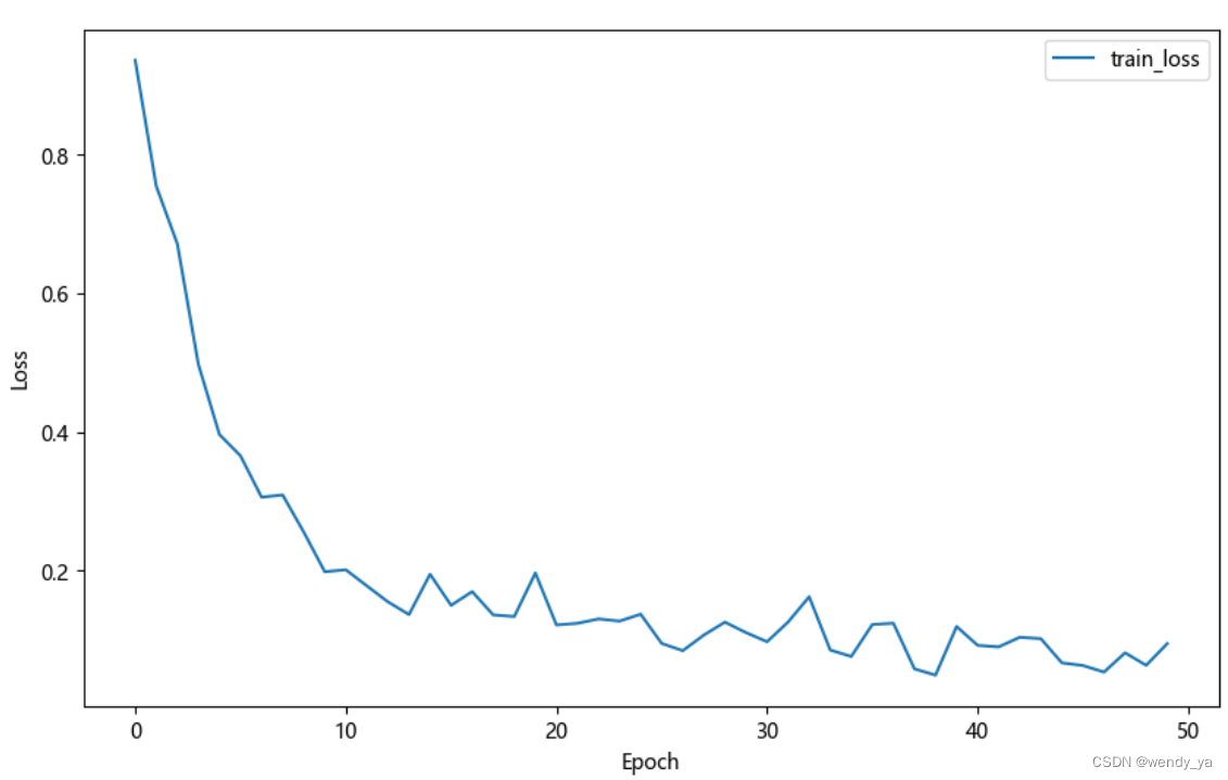
优化器利用的是Adam优化器,损失函数使用crossEntropy函数。
代码略
50个epoch的运行效果如下: